A novel clustering method - Crystal clustering

Python/Matlab code on GitHub repo

This clustering method, proposed by myself, is used in the climate classification.

Phenomenon

Imagine how a grain of sugar dissolves in water. Before it dissolves, the sucrose molecules form hydrogen bonds in between, so they condense as a macroscopic solid bulk.

The sucrose molecule (credit: UCLA chem)

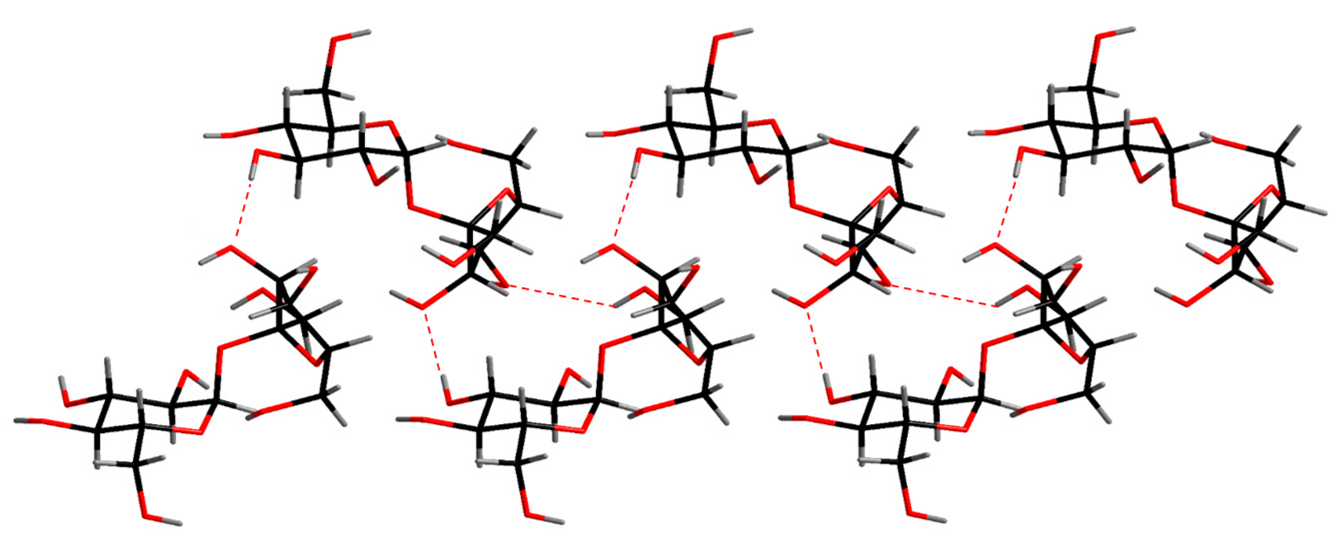
The crystal structure of sucrose (credit: Ji-Hun An et al. (2017)) The dashed lines show the hydrogen bonds.

Hydrogen bonds are what the sucrose molecules take to form the crystal structures. As a side note there’s also van der Waals force between the molecules.

When met with water, some of the hydrogen bonds break for water molecules cut in. Say there’s not enough water, and not all the bonds are broken. In this case, at the macroscopic level, the sugar is partially dissolved and there’s no ongoing net dissolution in the system, while at the microscopic level, the sucrose molecules in the aquatic phase occasionally collides with the ones on the edge of the solid phase, forming hydrogen bond and precipitates. Meanwhile, on the other side of the solid water molecules drag out the solid-phase-locked sucrose molecules. Microscopic dissolution and precipitation are happening simultaneously at the same speed, so the macroscopic observation is no net dissolution or precipitation.

If you can’t imagine that, this video (credit: Berean Builders) may help.

As the partial dissolution system stablizes (aka reaches equilibrium), it naturally forms several clusters of solid blocks. If we view the sucrose molecules as the data observations to cluster, now we get the result with outliers dissolved away (or as singleton clusters).

Modelling

But how can we model this process by computer algorithm? We need to dive deeper into the motive of this spontaneous process - what drives the bond to form/break?

For the sake of simplicity we will make certain assumptions, e.g. there’s no pressure-volume work in the process.

It’s the Gibbs Free Energy. The definition is

\[G=H-TS\]

where $H$ is the enthalpy (bond energy), $T$ is the thermodynamics temperature (always positive), $S$ is the entropy. A process is spontaneous in thermodynamics only if it results in a decrease in the system’s Gibbs free energy.

We keep the system at a pre-set temperature, so $T$ is a constant here. Whenever a bond breaks, the system absorbs energy ($\Delta H$ is positive), and the degrees of freedom increases ($\Delta S$ is positive), and vice versa. Whether this is thermodynamically possible depends on the condition - if $\Delta G = \Delta H - T\Delta S < 0$, it is. It’s easy to know that higher temperature favors bond breaking, leading to more clusters.

Next let’s define $H$ and $S$ in terms of the data clustering system. We have to define the system itself first.

This is a blog post, so I prefer to make it as simple as possible, using minimal math representations.

• Data obervations to be clustered: a $n$ by $m$ matrix $X$, rows are the observations and columns are feature dimensions. The observations can have different weights, $w_i$ for the $i$-th observation. This can be plotted as a graph $G$ with $n$ nodes. At this point let’s assume the graph is fully connected, and the edge weight is the distance in the feature space between the connected nodes. We also use the term bond in chemistry for graph edge, and form a bond for add/connect an edge, break a bond for remove/disconnect an edge.

Distance measures are not limited. Here we assume Euclidean distance.

• Clusters: connected components of the graph $G$. In this way only the minimum spanning edges (edges on the minimum spanning tree) matter, because non minimum spanning edges do not affect the connected components of the graph. From a viewpoint of the physical world, if a molecule in the aquatic phase choose to form a bond with a molecule in the solid phase, it would always prioritize the nearest one, resulting in a minimum spanning forest on the graph representation. So the fully connected graph reduces to a minimum spanning tree (MST) of $G$, denoted as $G_{MST}$.

The MST is similar to a single-linkage hierarchical clustering tree.

• State: The system evolves with bonds forming and breaking during the process before the stable state is reached. During the process, get a snapshot of the system, and we will have a subgraph of $G_{MST}$, with the same set of nodes and a subset of edges. The starting state is the connected MST, and there’s a potential ending state where all bonds are broken which is possible given a sufficiently high $T$.
• Action: A bond forming or breaking is called an action. An action that results in a decrease of the Gibbs free energy is called a feasible action.

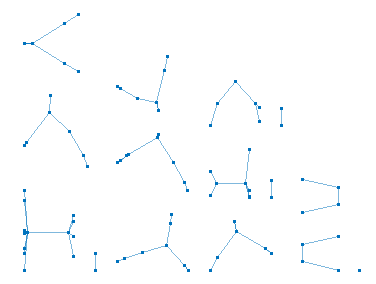
A state of the data clustering system

Enthalpy

For two data observations $X_i, X_j$ with weight $w_i, w_j$ and the distance between them is $d_{i, j}$, how do we define the bond energy between them? Here I would employ the concept in electrostatics:

\[\Delta H_{i,j}^{form} = - \frac{w_i w_j}{d_{i, j}}\] \[\Delta H_{i,j}^{break} = \frac{w_i w_j}{d_{i, j}}\]

This is analogous to the energy stored in a system of two point charges. The closer the two points are, the higher potential they form a bond in between ($\Delta H$ is more negative), and vice versa. The negative inverse manipulation emphasizes this effect for the points that are close enough. The value of $\Delta H_{i,j}$ is not dependent on the state of the system.

Under common scenarios we do not add up the weights of data observations in the connected component when calculating enthalpy. If we do so, it would produce a strong gravitational effect that draws a large number of data observations into one cluster, which, is a more faithful reproduction of the crystallization process (crystal growth after nucleation), but is not desired under the data clustering setting. What we want to simulate here is the system kept at the nucleation stage.

Weights are not considered in the following experiments. All observations are treated as equal weight.

As long as weight is not considered, the generated MST is the same as if Euclidean distance is directly used as the formula for bond energy.

We define the system enthalpy to be zero at the starting state where all bonds in the MST are connected. Enthalpy is summable with respect to bonds. For a certain state of the system, add up the $\Delta H^{break}$ of all bonds in MST which have broken and we get the enthalpy of the state. That is

\[H = \sum_{i, j \in e_{MST} \wedge i, j \notin e} \frac{w_i w_j}{d_{i, j}}\]

Entropy

For a state with $k$ clusters and each cluster $i$ has data observations whose weights sum up to $c_i$, the entropy is calculated as

\[S = \frac{1}{N} \sum_{i=1}^k c_i \log \frac{c_i}{N}\]

where $N = c_1 + c_2 + … + c_k = \sum_{j=1}^n w_j$. This is from the definition of information entropy.

It seems non-trivial to efficiently calculate the entropy change of an action ($\Delta S_{i,j}$). A brute-force algorithm is to calculate the entropy of the state before the action and that after the action, and then subtract, which is $O(n)$ time complexity. We may also utilize data structures for dynamic trees, e.g. the Link/cut tree, which can reduce the time complexity to $O(\log n)$ for this step. Unlike enthalpy change, this value is dependent on the state of the system.

The $\Delta S$ is sometimes called information gain.

Algorithm

We are going to solve the optimization problem on $G_{MST}$. Remove some edges of $G_{MST}$, so that

\[f(G_{MST}, T) = H - TS\]

is minimized. $T$ is a given positive constant (hyperparamter). $H$ and $S$ are defined above.

The Matlab code provides four algorithms, three of which are experimental and for research purposes. Here I would only introduce the greedy-backtrack algorithm, which is the go-to algorithm in most cases. This algorithm simulates the precipitation-solubility equilibrium.

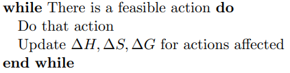
The description is self-explanatory and I would rather not dive into the details here. Interested readers may check the commented code. One thing to note is that the algorithm does not guarantee to converge nor to find the global optimum (aka the thermodynamically stable state), but in most cases it converges fast and the result is good enough to use (or even preferred over the thermodynamically stable state, as we can see in Sec 6). The bottleneck of the algorithm lies in calculating the pairwise distances between observations and constructing the MST, which demands $O(n^2)$ time and space. The running time also depends on the value of $T$: a higher $T$ means more actions before convergence and thus more time. Each action is $O(n \log n)$ with link-cut tree.

Why is this algorithm not guaranteed to find the global optimum? It’s easy to understand by physical chemistry. Some reactions, e.g. hydrogen reacting with oxygen to produce water, though thermodynamically possible (the energy of the product state is lower than the energy of the reactant state), only happen under certain conditions, e.g. ignition. Ignition provides the initial energy to induce the reaction. The necessary amount of energy is called activation energy. Or, there’s some other reactant (catalyst) in the system which provides a shortcut reaction mechanism that gets around the energy barrier for the reaction to happen. On the other hand, from the viewpoint of data science, this can be understood by analogizing to gradient descent. This greedy algorithm is similar to gradient descent, which may stuck into a local minimum, and in this situation some momentum is needed to get over the local minimum and continue the search. We will showcase this situation in Sec 6.

Experiment

On the Iris flower dataset, the clustering results are shown as follows. For illustration purpose, we only work on the 102 unique combinations of the last two dimensions. It’s clear that number of clusters increases with rise of temperature.

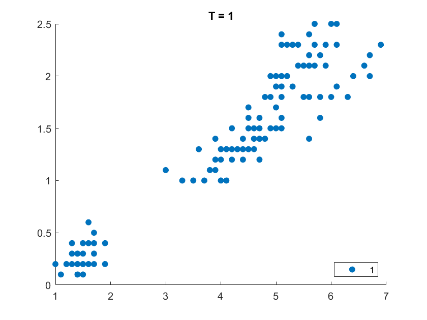
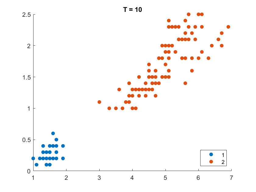
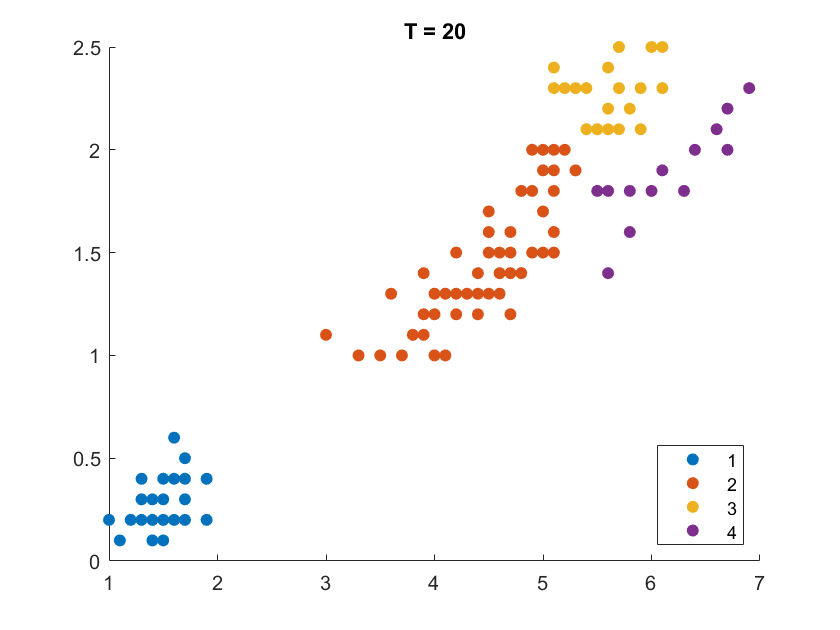
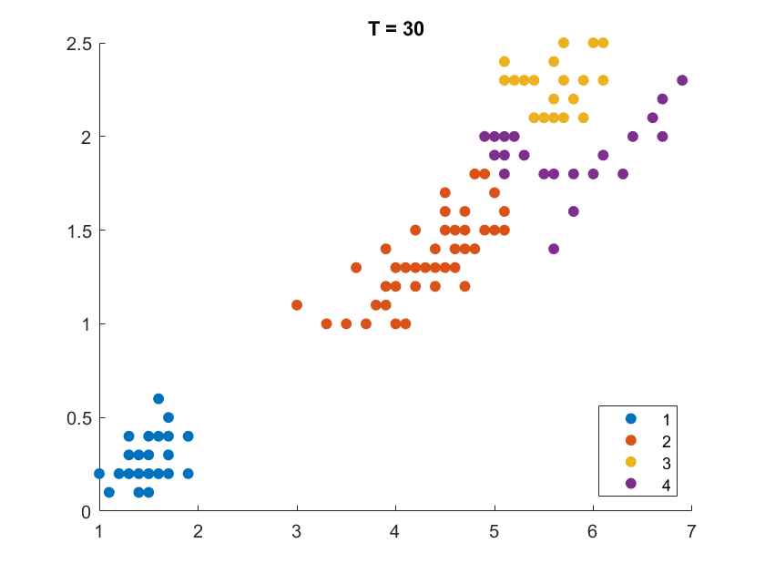
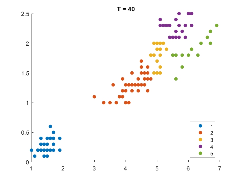
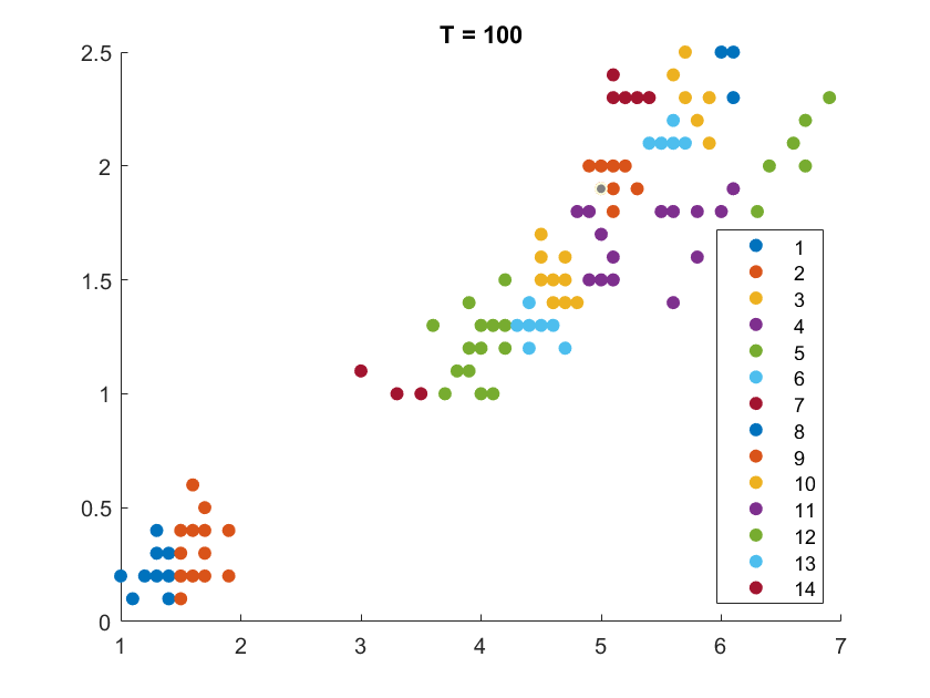
More details are elaborated in Sec 6 based on the climate cluster centroids dataset. There we can see $T$ not only controls the number of clusters, but also affects their morphology. This can also be obsereved from the different results of $T=20$ and $T=30$ on the Iris example.

The algorithm is benchmarked on 73 datasets described by Marek Gagolewski using the clustbench package and achieves very high score. Details are in the Github repo.

Theoretical temperature and the scale of data

There are two extreme states of the system - the starting state where no bond in the MST is disconnected (so there’s only one cluster), and the ending state where every bond is disconnected (so there are $n$ clusters that each observation is a singleton cluster). It’s certain that given $T=0$ the system will stay in the starting state, but what is the minimum $T$ that allows the system to evolve into the ending state?

Say at a certain temperature $T_{theo}$, the system evolves from the starting state to the ending state which is the global optimum. The $\Delta G$ of this process is

\[\Delta G = \Delta H - T_{theo} \Delta S = \sum_{i, j \in e_{MST}} \frac{w_i w_j}{d_{i, j}} - T_{theo} \log N\]

It’s a bond-breaking process so both $\Delta H$ and $\Delta S$ are positive. The maximum entropy for the system is $\log N$, and $N = \sum_{j=1}^n w_j$.

At the thermodynamically stable state, we have $\Delta G = 0$, so

\[T_{theo} = \frac{\sum_{i, j \in e_{MST}} \frac{w_i w_j}{d_{i, j}}}{\log N}\]

This is the value of $T$ that thermodynamically (or say theoretically) guarantees the system evolves into the ending state. But the evolution may not be possible by kinetics, which means the greedy-backtrack algorithm may not discover the ending state. More often than not it cannot.

The theoretical temperature of the Iris flower dataset is calculated to be ~179.8. Our experiment showed given $T=180$, the system evolved into a state of 27 clusters instead of the theoretical 102 clusters based on the greedy-backtrack algorithm.

So what does the theoretical temperature tell us? As far as I know it provides a hint of the scaling of the parameter $T$ on the given dataset. So we can better estimate an initial value for trial by knowing its order of magnitude - whether we should start the trial from some value below ten, or some tens, or some hundreds. We can also define a standardized situation where $T_{theo} = 1$, so that for any dataset the temperature scale is mostly the same. By our experiments, a rule of thumb is that the theoretical temperature will give ~ $0.3N$ clusters ($N$ is the number of points in the dataset).

Further Information

This method actually belongs to a group of clustering algorithms of optimising different criteria – divisive strategy over MST named by Marek Gagolewski et al. (2023). In the article they comprehensively studied the clustering algorithms based on MST and compared with traditional algorithms like $k$-means, BIRCH, linkage, PAM, etc. They concluded that MSTs are suitable for representing dense clusters of arbitrary shapes, and are relatively robust to outliers in the outer parts of the feature space.

This method is out of their scope of study because it normally does not accept a fixed number of clusters $k$ as input. Rather, we use a relaxation strength parameter $T$. This can have its own pros and cons. $k$ is more intuitive to humans, while the good things are

• the scale is continuous, unlike $k$ has to be an integer
• easier to deal with outliers, no need to investigate the number of outliers for a good guess of $k$
• good for the situations where the target $k$ is not known beforehand

It may need more trial and error to get the best $T$ for the desirable outcome.

In terms of the physical world, $T$ involves everything that moves the equilibrium, not only temperature. For example in the solubility scenario it can point to the amount of solvent - with enough water sugar can be totally dissolved, which corresponds to a very high $T$ so that every data observation goes into a singleton cluster. Relaxation strength can better describe this parameter. The physical phenomenon is more complex than what is discussed above, and there’s no need to dive into individual factors that affect the equilibrium to introduce the clustering method.

The most similar method discussed by Marek Gagolewski et al. (2023) is ITM by Andreas C. M¨uller et al. (2012). Their method requires the number of clusters $k$ as input and targets at maximizing the mutual information between input data and output labels. Following a similar greedy MST-cut approach, it focuses on intra-cluster entropy instead of our inter-cluster (intra-system) entropy.

This method may also have more advanced applications, such as a multi-stage clustering process which simulates the fine fractionation operation in chemical production: at a higher temperature, the first aggregated cluster is removed from the system, and then gradually cool down to remove the subsequent clusters step by step at different levels of temperature. The gravitational effect of agglomerated weight is yet to be further explored and may have its potential applications.