A neural network approach for climate classification - Sec 6. 533 SOM and crystal clustering

In Sec 3 we used a 322 SOM and did a simple clustering. The resulting scheme is clear and concise, but at a sacrifice of granularity - there’s even not a subtropical climate type which is often not negligible. So we are going to derive a climate classification scheme with more details. This section will focus on the methodology. Next section will focus on interpretation of the climate types.

533 SOM

Recall the climate features we analyzed in Sec 3. The standard deviation of the three features are 5.41, 3.66, 3.39 respectively. Aside from 3:2:2, it’s also acceptable to approximate the ratio as 5:3:3. Intuitively, this dilineates the globe into tropical, subtropical, temperate, subarctic and arctic - five thermal zones. Continentality and seasonality are also divided into three levels each.

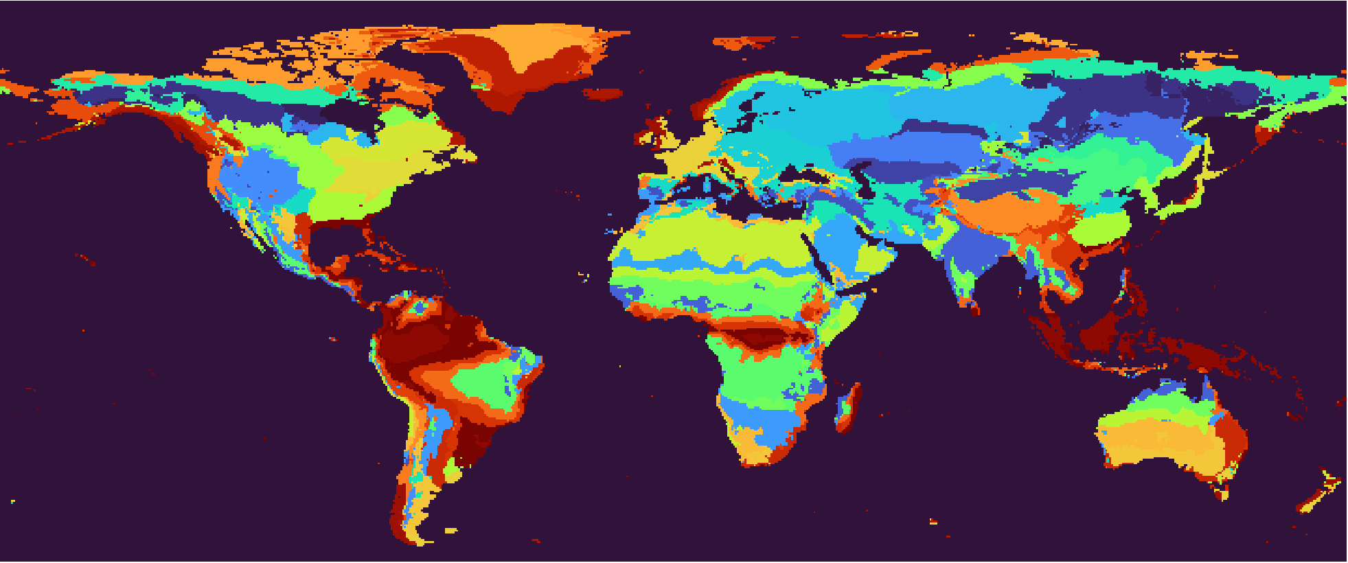The result of 533 SOM, 1991-2020 climate normals. Right-click for full image.

Using this 533 SOM, we will have 45 climate types as shown above. The Köppen scheme defined 30 climate types, and even that seems a bit excessive. Also in many cases it may sound redundant to have three seasonality levels like non-seasonal, slightly seasonal and significantly seasonal.

It turns out that we don’t need the same granularity on the continentality-seasonality plane for all temperature levels. In the coldest arctic zone, it doesn’t matter for plant growth whether the climate is seasonal or continental - the coldness dominates everything. The need for granularity increases with temperature level. But the SOM is a rigid hexagonal grid which cannot be customized in this way, so we see a fractionated interior Greenland in the result.

We need a way to merge the fractionated climate subtypes into a reasonably compact climate classification system, meanwhile preserving the unique climate characteristics for each individual type. The task is a clustering on 45 observations with 15 features.

Though we only analyzed the top 3, we are actually working on 15 climate features, as noted in Sec 3.

The dataset is provided as centroids.mat in the Crystal Clustering code repo.

Why crystal clustering?

Ward hierarchical clustering

Seeing that the number of observations is small, typically we first use the Ward hierarchical clustering tree to have a visualization of the data structure.

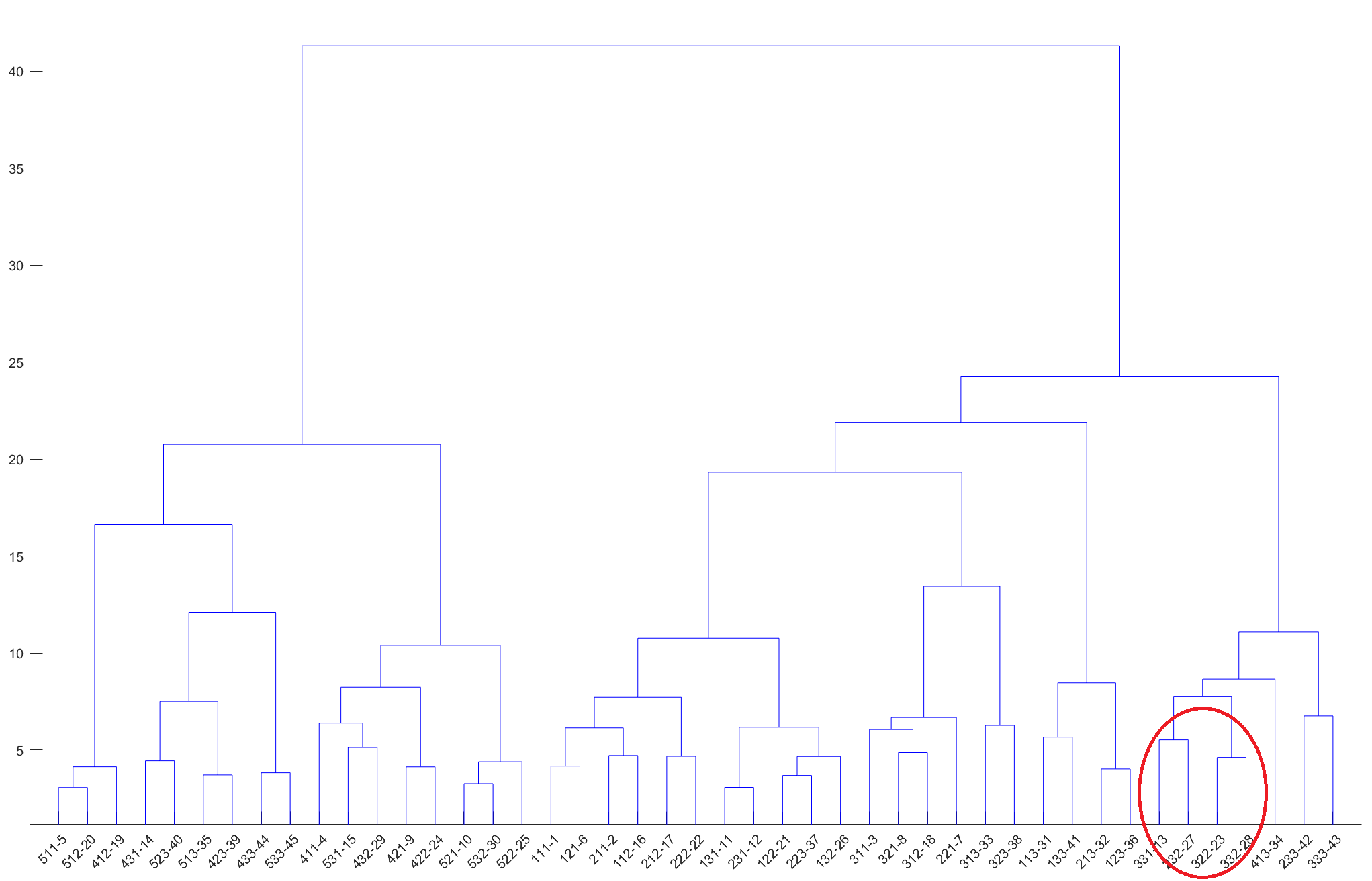The dendrogram of the 533 SOM subtypes. Right-click for full image.

To show how crystal clustering is different from other clustering methods and is especially useful here, we will focus on the red circled part. Four subtypes are involved: 322-23, 332-28, 331-13, 232-27. In this naming convention the first three numbers are the coordinates in the SOM grid and the number after the hyphen is a linear index.

As discussed in Sec 3, the first coordinate indicates the thermal zone (increases with coordinate), the second coordinate indicates continentality (decreases with coordinate) and the third coordinate indicates seasonality (decreases with coordinate). The directions of the coordinates can be different in multiple trainings of the SOM.

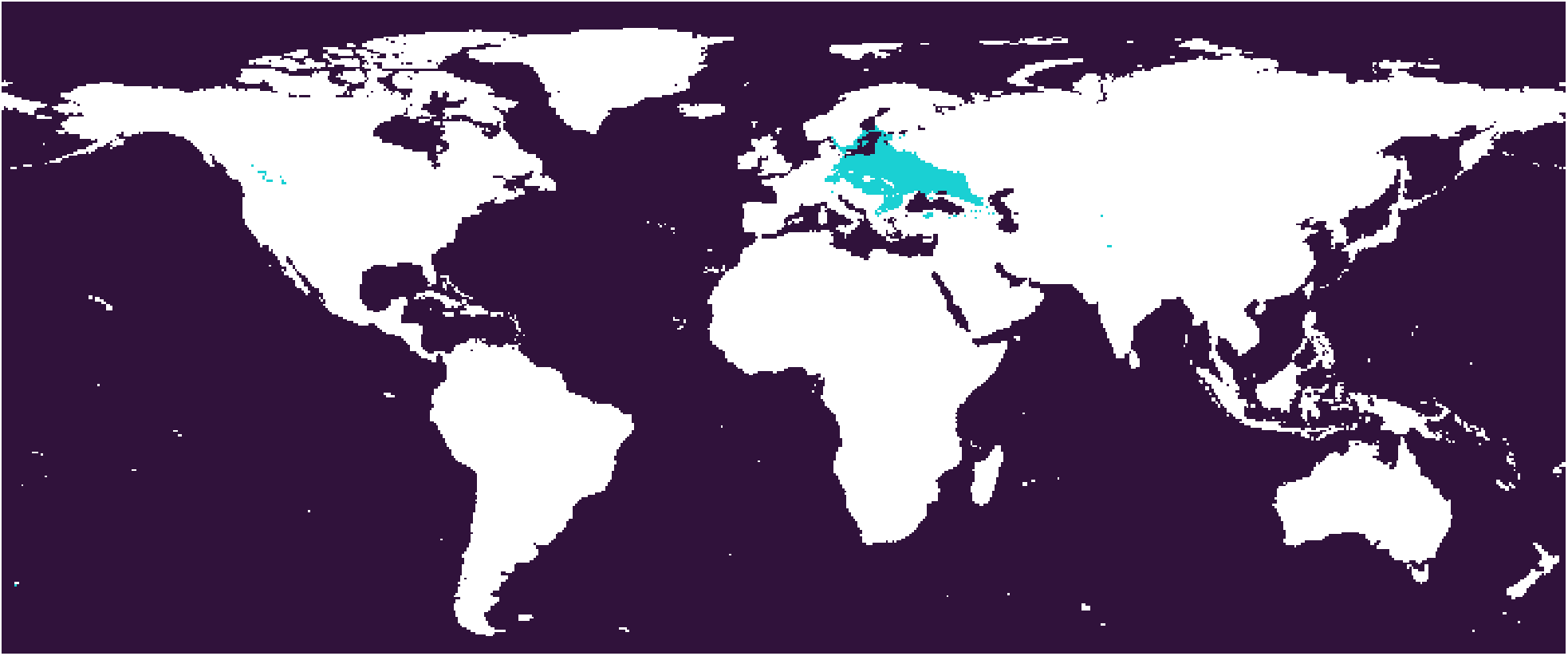
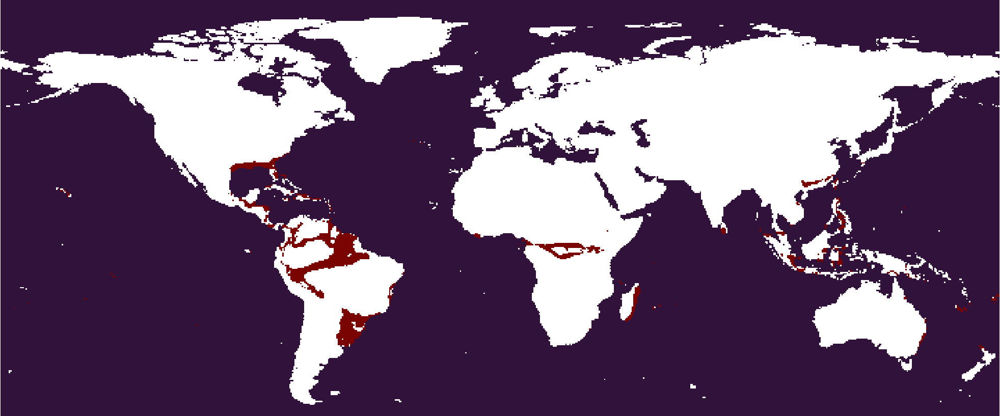
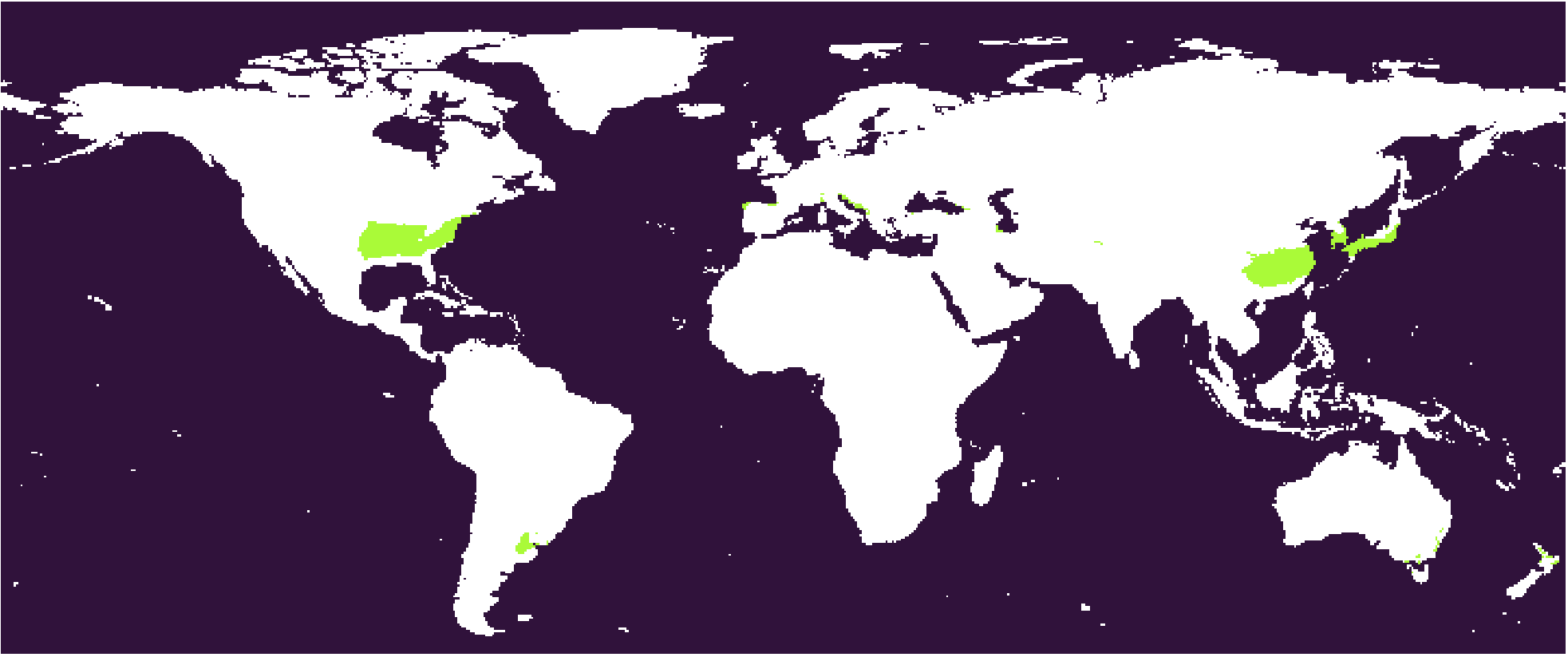The 322-23 subtype. The humid subtropical type, largely equivalent to Köppen’s Cfa.

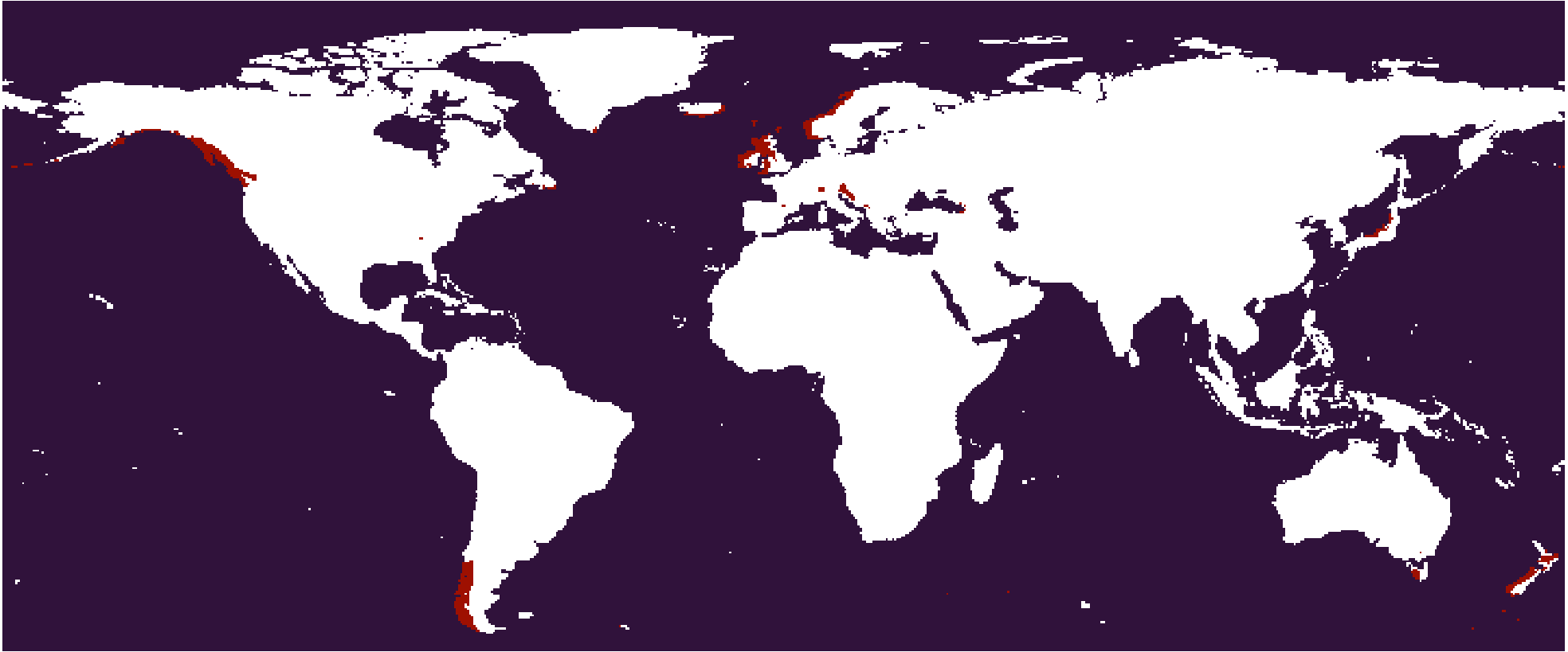
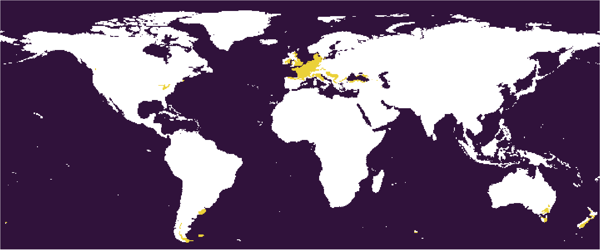The 332-28 subtype. The West Europe type. Cfb in Köppen scheme.

The 331-13 subtype. The Central Europe type. Cfb in Köppen scheme.

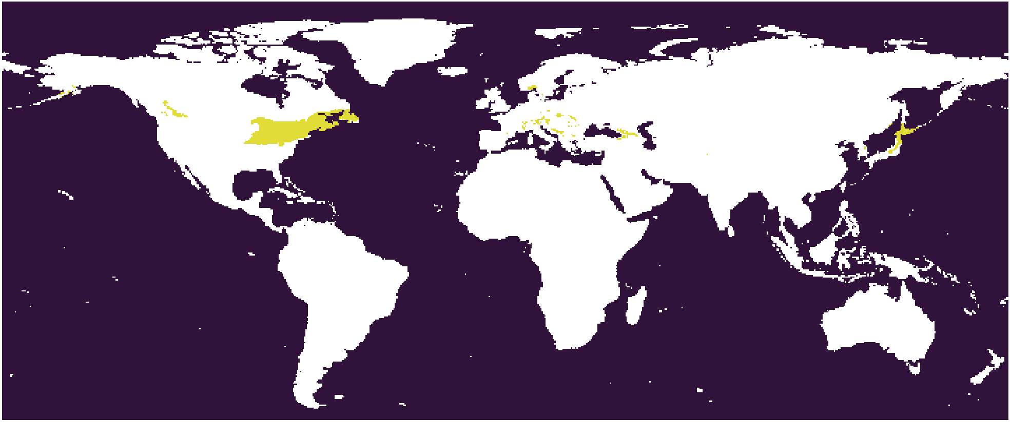The 232-27 subtype. The Northeastern US type. Dfb in Köppen scheme.

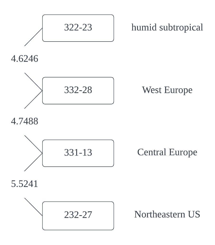The pairwise distances between the cluster centroids in the feature space.

The distance between 322-23 and 332-28 is the closest, so this pair is connected in the linkage tree first, and then 331-13 and 232-27 are paired. This is the logic of the linkage tree. Based on this tree, the paired subtypes may be merged or not according to the desired granularity, but a cross merge is not allowed, e.g. 332-28 merging with 331-13. This kind of cluster organization does not agree with traditional climate classification schemes and common knowledge - usually the Europe is deemed as temperate zone while 322-23 is subtropical, and the 232-27 is much colder. If we simply merge 322-23 and 332-28 according to their proximity, we are going to lose the layered thermal zone structure.

Crystal clustering

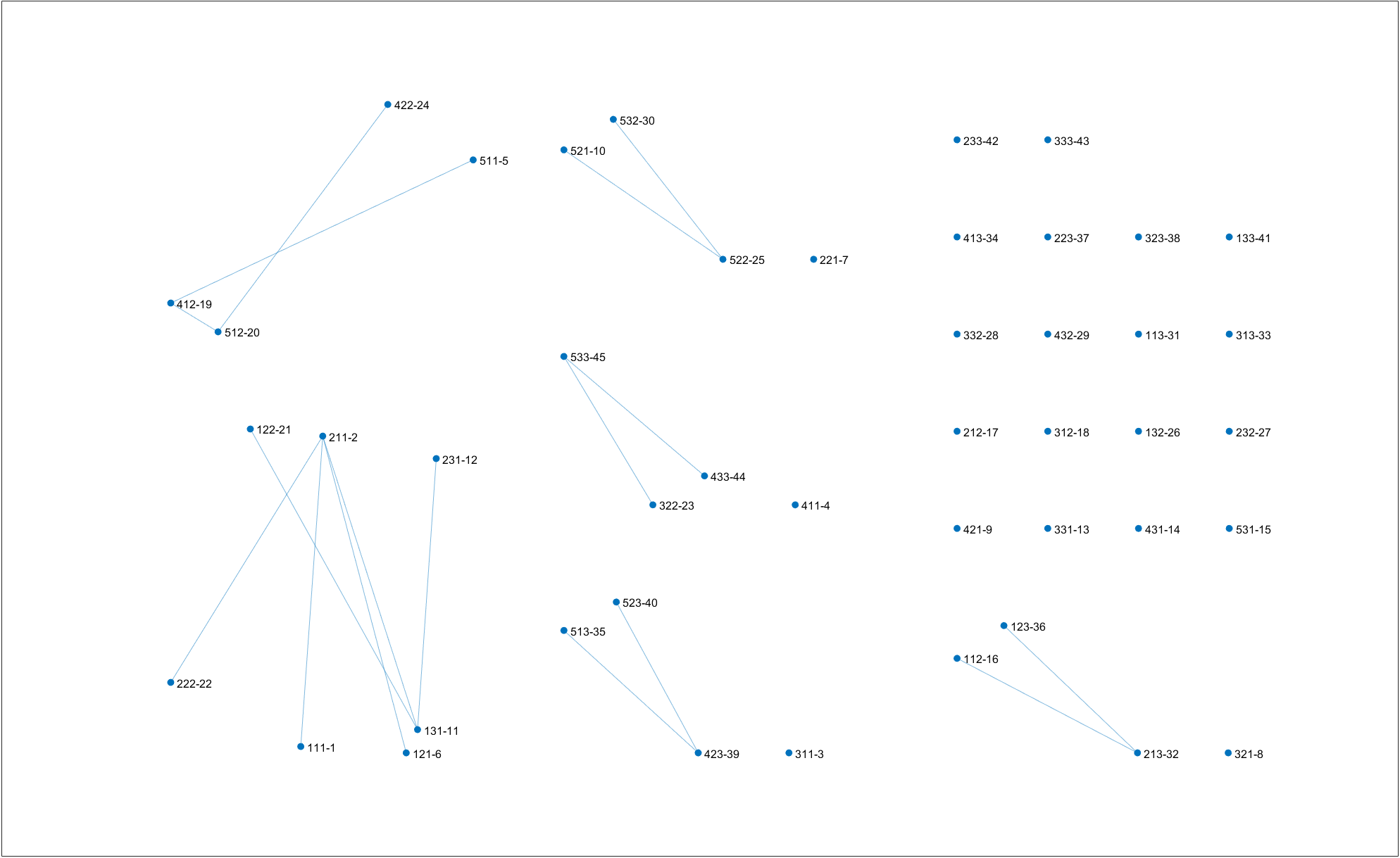
Crystal clustering is run on the 45 cluster centroids given $T=5.2$. The minimum spanning tree and the order of bond breaking are visualized below.

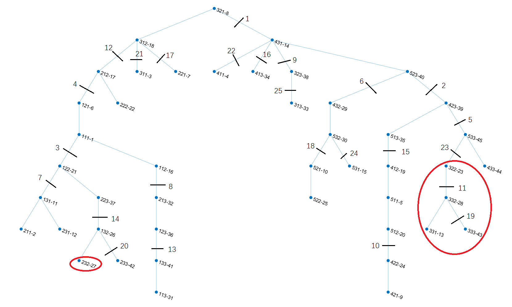
In this figure the length of the bond does not reflect the distance between cluster centroids in the feature space. Right-click for full image.

The MST forms a nice structure that reflects the intrinsic topology of the climate space - broadly speaking, the 1 and 2 thermal zones (cold) sit in the left branch, the 4 and 5 thermal zones (warm) sit in the right branch, and the 3 thermal zone (temperate) sits in between. It appears like the histogram of the first principal climate feature shown in Sec 3.

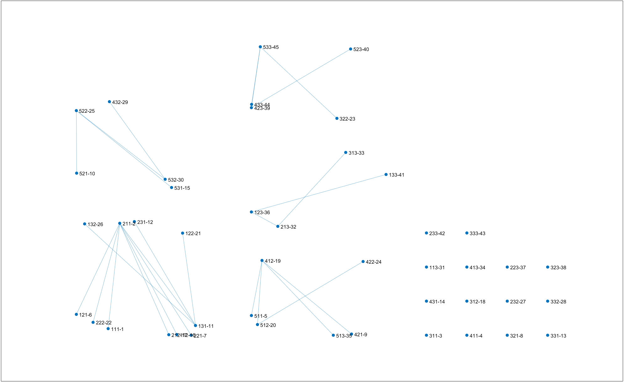
The subtypes in the big red circle are an exception. It’s tricky that their growing condition is closer to those in the 4, 5 thermal zones, so they are branched on the right side. During the run of the greedy-backtrack algorithm, after the fifth bond break, the structure as shown in the below figure is left out.

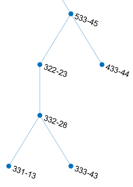
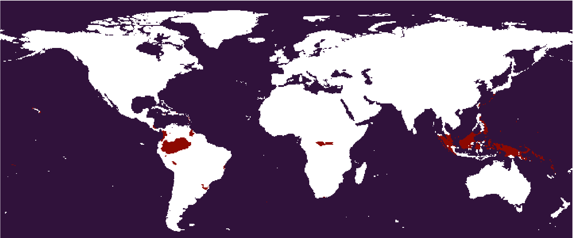
The 533-45 subtype. Largely Af/Am in Köppen scheme.

The 433-44 subtype. Af in Köppen scheme.

The 333-43 subtype. Dm in the 322 scheme.

Even though the distance between 332-28 and 322-23 is slightly closer to that between 332-28 and 331-13, the algorithm chooses to break the former first. It’s due to the effect of entropy. Breaking the former bond gives a 3-3 separation over the six types, while breaking the latter gives a 1-5 separation. The former action results in a higher increase in entropy. In terms of climatology, this action separates the humid temperate zone (the lower section of 332-28, 331-13 and 333-43) with the subtropical-tropical humid zone (the upper section of 533-45, 433-44 and 333-43). It’s a separation of higher level that should be done over that on the lower branch which gives details. This action takes into consideration not only the distance between two observations, but also the structure of surrounding connected components. This explains the role of entropy in crystal clustering.

What about the 232-27? It’s on the left branch (which represents the cold zone), not engaging with those humid temperate types at all! Upon the MST is built, 232-27 is differentiated. Given the observations not on the same branch of the MST, there’s no chance that they are assigned in one cluster. This ensures that the data organization found by the MST is preserved in the clustering result.

The Ward linkage tree is different from MST in that whenever two observations are connected, they form a new cluster with a new cluster centroid. However when constructing the MST, the observation is always at its original location in the feature space. This difference leads to different data organizations. The $k$-means clustering, implemented in a non-hierarchical manner, has the same objective with Ward linkage tree that minimizes the total within-cluster sum of squares. These methods don’t engage much with the topology of clusters in the feature space.

To sum up, crystal clustering follows SOM’s idea of structurization of clusters and is very suitable as a postprocessing method when topology of clusters is a concern. SOM plus the crystal clustering can be a potentially useful manifold learning method.

Kinetics in crystal clustering

Still on the red circled structure. Given $T=5.2$, the system finally evolves into a state of 26 clusters, where the three subtypes 322-23, 332-28 and 331-13 form a 1-2 separation - the latter two are connected.

It’s easy to see that a state with lower $G$ exists - the former two connected and 331-13 isolated, because the entropy is the same for the 2-1 state, but the bond energy between 322-23 and 332-28 is higher than that between 332-28 and 331-13 (a higher bond energy means a closer proximity in the feature space). But it’s not possible for the system to reach that state under this condition, as is shown below.

There are two proposed routes to reach that state:

• 332-28 first connects with 322-23, then breaks with 331-13
• 332-28 first breaks with 331-13, then connects with 322-23

As an example, let’s calculate the $\Delta G$ of 332-28’s connection with 322-23.

\[\Delta S = S_{end} - S_{start} = -\frac{3}{45} \log \frac{3}{45} - (-\frac{2}{45} \log \frac{2}{45} - \frac{1}{45} \log \frac{1}{45} )=-0.0424\] \[\Delta H = - 1/d = - 1/4.6246 = - 0.2162\]

Bond connection always has a negative $\Delta H$ and a negative $\Delta S$.

\[\Delta G = \Delta H - T \Delta S = -0.2162 + 5.2 * 0.0424 = 0.0043\]

A positive $\Delta G$ means the action is not possible. Similarly we know that 332-28 is not possible to break with 331-13 under the given $T$.

Kinetics hold the system on a state with higher energy. But that state is even preferred over the state with lower energy (aka thermodynamically more stable state), because it’s more structured. As the above analysis shows, the breaking between 332-28 and 322-23 is significant.

Given $T=5.0$, the first route will get executed in the algorithm run. Besides, the system will not go over the last two breaks (24th and 25th). In this sense, $T$ not only controls the number of clusters, but also affects their morphology. This is shown in the example in the Python code.

Shifting the value of $T$

The theoretical temperature $T_{theo}$ for this dataset is ~2.6. Here we make a comparison of the clustering results on $T=5.2, 3.0, 2.6$ respectively. $T=3.0$ is an important threshold in that it’s the maximum temperature to have no singleton cluster on this dataset. The algorithm starts to recognize outliers above this temperature. It’s another number worth exploring other than $T_{theo}$ while working with real-world datasets.

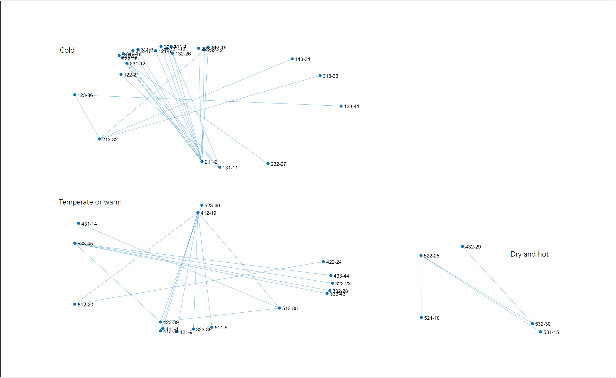
Clustering result on $T=5.2$. Cluster names are going to be explained in Sec 7. Right-click for full image.

Clustering result on $T=3.0$. Right-click for full image.

Clustering result on $T_{theo}=2.6$. Compared with $T=3.0$, Gh is merged with Fsk. Right-click for full image.

Weight effect

What if we assign weights to the observations? It makes the mechanism drastically different. Here the weights are given as the land proportion of each 533 SOM subtype. The $T_{theo}$ of the weighted dataset is ~3.7.

Clustering result on $T=5.2$. The six types of the 322 scheme, named in the image, are largely produced. Right-click for full image.

Clustering result on $T=5.0$. Right-click for full image.

Clustering result on $T_{theo}=3.7$. Right-click for full image.

Clustering result on $T=1.6$. This is the maximum temperature to have no singleton cluster. The result looks like a high-level hierarchical clustering. Right-click for full image.

It can be seen the weights favor the formation of large clusters (crystal growth) and discourage the linkage of single observations (nucleation). Just weights assigned; we don’t add up the weights in the calculation of bond enthalpy when observations are linked to be a cluster. It’s a phenomenon for further research; for now, under common clustering scenarios, the effect seems undesired.

It’s worth noting that compared with the result of $T=5.2$, the algorithm gives one more cluster on $T=5.0$. This situation is not common. Analogously, some substances have lower solubility on higher temperature, like calcium hydroxide in water. Also the cluster morphology has noticeable differences in the two results.