Van's homepage
A child exploring the world alone.
A neural network approach for climate classification - Sec 1. Vegetation mapping methodology
by Van
The preface introduced the idea of empiric climate classification, the Köppen example and the skeleton of our approach. Put simply, the approach consists of two steps: first, learning the mapping from climate normal data to vegetation distribution data by a neural network (NN), and then clustering on the climate features learned by the NN. This article discusses the methodology of the first step, mainly the dataset and the NN structure.
In this article series the terms vegetation and land cover are used interchangeably. The two terms do have moderately different meanings but omitting the difference turns out to be safe for our methodology.
Dataset
Summary of the datasets.
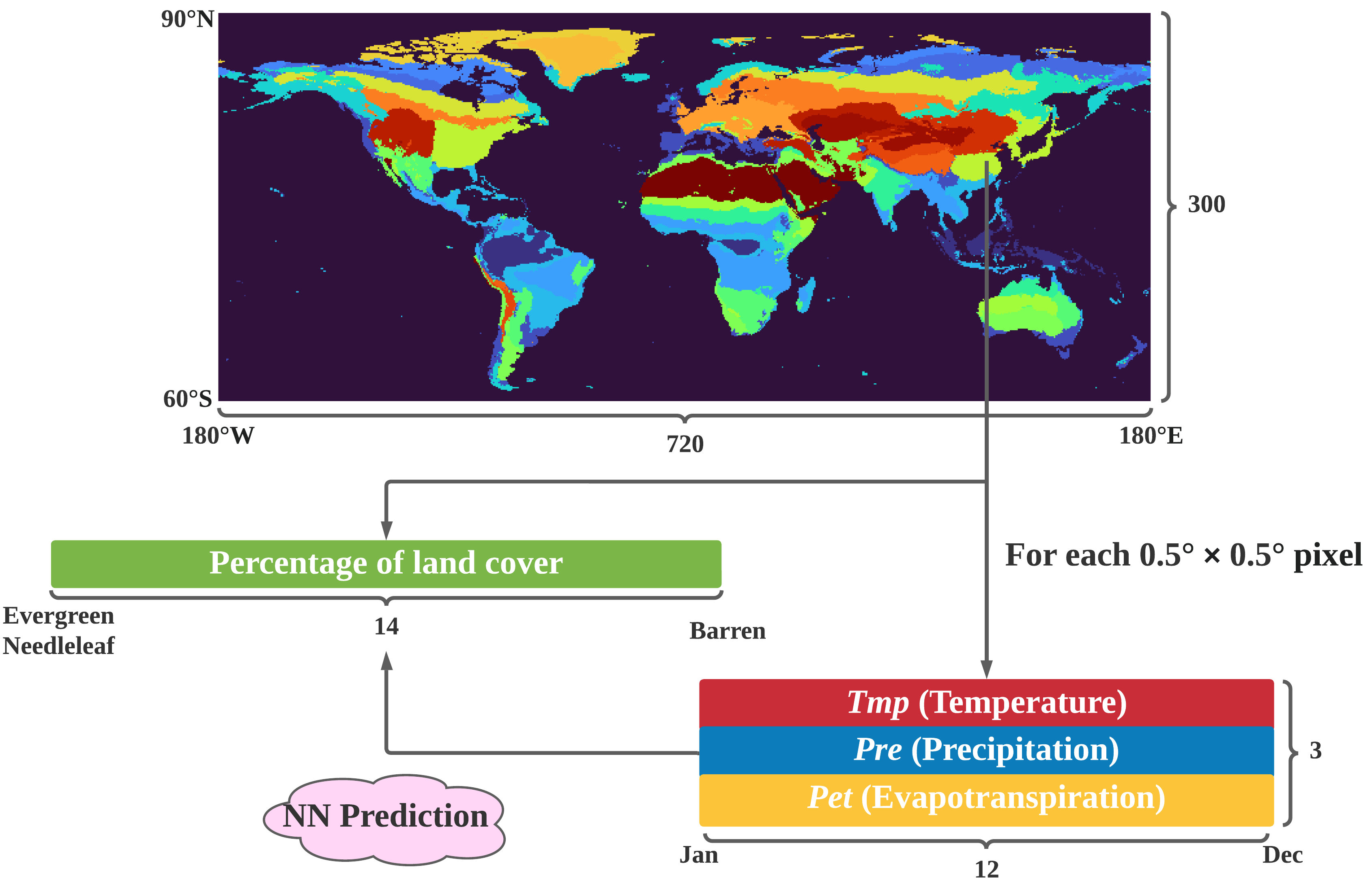
The land cover dataset is the prediction target for the neural network while the climate normal dataset serves as the network’s input.
Land cover data
The MCD12C1 v6.1 dataset (Antarctica excluded) is taken to construct the land cover dataset. The cover percentage of each IGBP class is used. The original dataset specifies 17 land cover types whereas some of them are considered not closely related to climate. We ignored the types of water bodies and urban and built-up lands, and merged croplands and cropland/natural vegetation mosaics into one. So there are 14 land cover types in our dataset. The original resolution is $0.05° \times 0.05°$. It’s spatially aggregated to $0.5° \times 0.5°$ to align with the climate normal dataset. The constructed dataset has 66,501 records, and each single record is a normalized $1 \times 14$ vector. Each vector entry stores the percentage of a certain land cover type on the $0.5° \times 0.5°$ land area with water or city covered area excluded.
For the definition of each land cover type, see Damien Sulla-Menashe and Mark A Friedl, 2018.
IGBP, the International Geosphere-Biosphere Programme, has closed in 2015. The website remains available until 2026. Most of its projects and networks have moved to Future Earth.
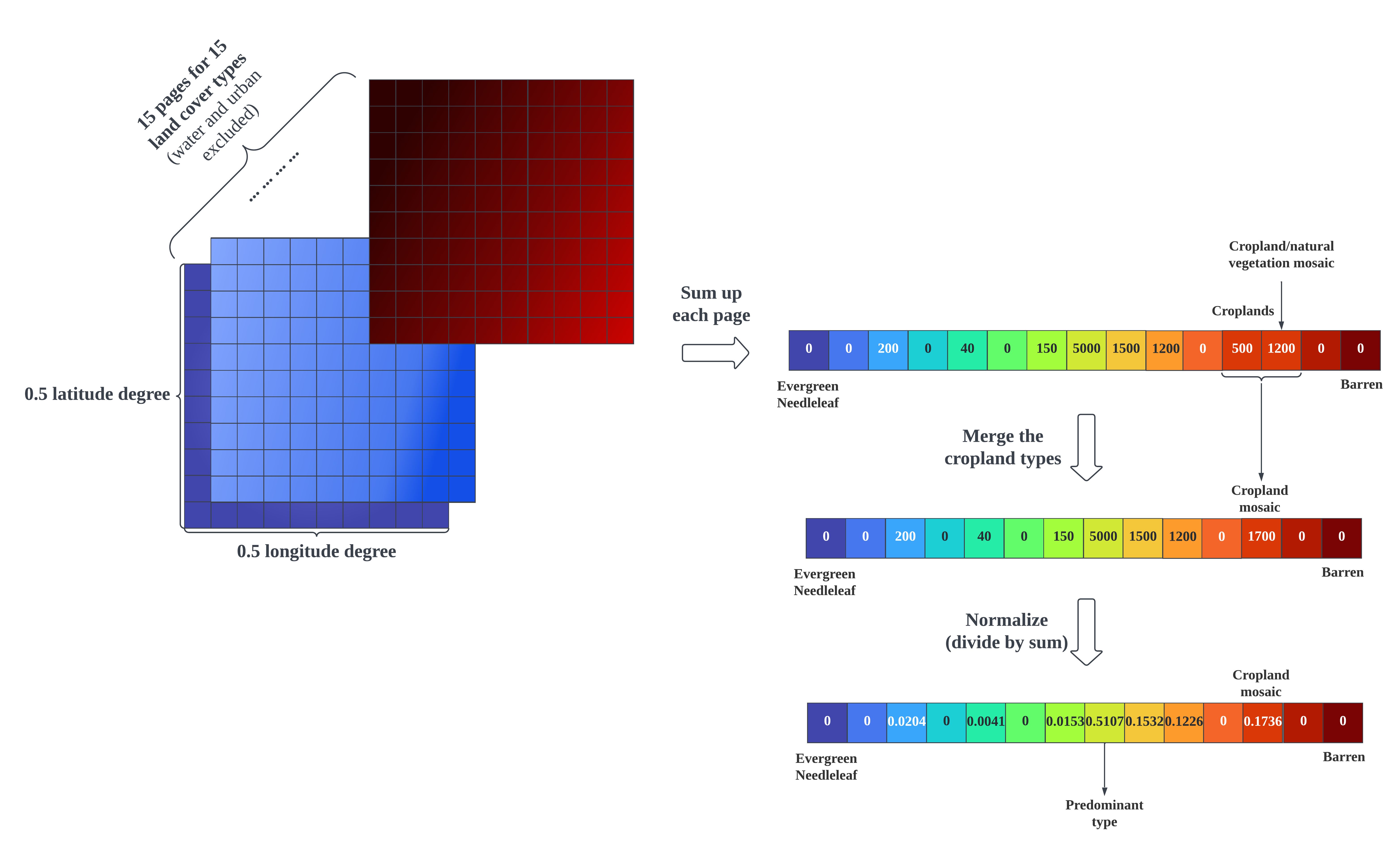 The land cover data calculation process. A cell on a data page stores the percentage of a land cover type on the specific $0.05° \times 0.05°$ area. Right-click for full image.
Climate normal data
The dataset we use is CRU TS v4.07. Three variables TMP (temperature), PRE (precipitation), PET (potential evapotranspiration) are involved. The CRU TS dataset covers global land excluding Antarctica at $0.5° \times 0.5°$ resolution, and the temporal granularity is one month. For each of the three variables, average on each month (Jan, Feb, …, Dec) through a period of 30 years, and a $3 \times 12$ matrix is obtained for each land pixel. The constructed dataset has 66,501 records (sea and Antarctica excluded, matching the constructed land cover dataset), and each single record is a $3 \times 12$ matrix.
Of the 66,501 records, there are ~46 (varies by year) records whose land cover vector is invalid (the whole area is lake or city). These records are not fed into neural network training, but their features are extracted by the trained network and taken into clustering afterwards.
Training set and validation set
At the time when this research was done, the MCD12C1 product contained data for the years 2001 to 2021. Given that the natural vegetation responds slowly to climate change, we use the climate normals of the years $(T-29)$ ~ $T$ (both ends included, so it’s a 30-year period) to predict the land cover of the year $T+1$. For example, use the 1991-2020 climate normals to predict the land cover of 2021. $T$ ranges from 2000 to 2020 which is a total of 21 years, so we have around $21 \times (66501 - 46) = 1395555$ instances of training data. Each instance is a $3 \times 12$ matrix of climate normal data paired with a $1 \times 14$ vector of land cover data. The last year’s data is used as the validation set, i.e. 1991-2020 climate normals paired with land cover of 2021.
The MCD12C1 dataset has been updated for the year 2022 on Sept 5, 2023.
The neural network
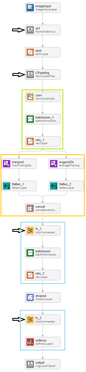
NN structure. Green box shows the convolution block, yellow box shows the pooling block, and blue box shows the regression blocks. Important layers are pointed to by the arrows.
The network, inspired by Köppen’s empirical rules, can be regarded as a spanning space for the empirical rules, and training the network is to find the set of rules that best describes the mapping between climate and land cover conditions. Here I would mainly introduce the special custom layers; for details of other layers, interested readers may check net.mat in this repo.
Custom activation layer
The custom activation layer act takes a $3 \times 12$ matrix as input. Together with the tanh activation layer that follows, it simulates empirical comparison of monthly TMP, PRE, PET data against certain thresholds (denoted as $\mu$ e.g., in Köppen scheme, the $0°$C threshold that distinguishes between C and D groups, the $18°$C threshold that distinguishes between A and C groups, etc.) by hypertangent function:
It can be regarded as a special row-wise $1 \times 1$ convolution or normalization, as shown in the figure below:
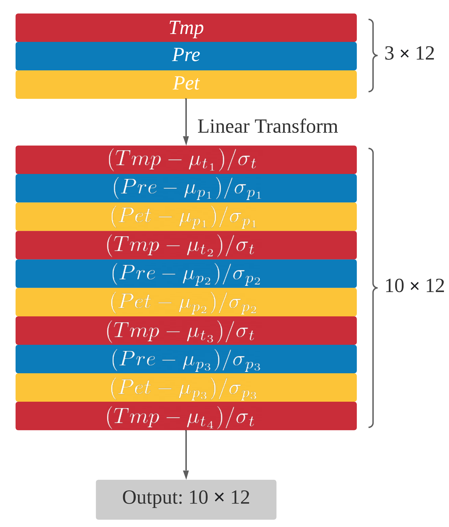
There are four thresholds for temperature ($\mu_{t_1}$ to $\mu_{t_4}$, initialized as -18, 0, 10, 22) and three thresholds for precipitation and evaporation ($\mu_{p_1}$ to $\mu_{p_3}$, initialized as 10, 40, 100). The $\sigma$s specify the sensitivity of each threshold. All temperature levels share a $\sigma_t$ which is initialized as 4 and for the three precipitation levels from low to high, $\sigma_{p_1}$ to $\sigma_{p_3}$ are initialized as 10, 20, 30 respectively. These parameters scale differently from other learnable parameters which are normally within $[−1, 1]$ in the neural network, so learning rate factors are assigned. Specifically, the learning rate for temperature related parameters ($\mu_{t_1}$ to $\mu_{t_4}$ and $\sigma_t$) is 30x, and the learning rate for precipitation related parameters ($\mu_{p_1}$ to $\mu_{p_3}$ and $\sigma_{p_1}$ to $\sigma_{p_3}$) is 200x, compared to other parameters in the neural network.
It is more flexible and intelligent to let the network learn these thresholds and scales on its own rather than assigning by human estimation. In addition, hypertangent activation is smoother than 0-1 thresholding as in empirical rules. We set a shared $\sigma$ for temperature levels based on the result of experiment. According to our experiment, when four different parameters are set, after training, their values appear very close. In this case it’s better to have fewer parameters for a simpler model.
Circular padding layer
The circular padding layer CPadding replicates the column of January behind that of December, and vice versa. Observing the natural repetition of years, this manipulation ensures that every month is equally represented in the following convolutions.
Convolution layer
The convolution layer conv has 32 kernels and the kernel size is $3 \times 3$. In this sense the receptive field of each kernel covers one season (three months).
Pooling
The max and average pooling layers have a pooling size of $1 \times 12$ to pool across all the 12 months. By this setting, convolved 3-month features are chronologically aggregated as min/max/average statistics over a whole year, and the season inverse between Northern and Southern Hemisphere is eliminated.
After pooling the annual features are flattened to 1D and concatenated to have the 512 features fed to the regression block.
The blocks described above can be substituted with a GRU/LSTM layer with $m$ hidden units, which takes the standardized $3 \times 12$ climate normal matrix as input (3 channels, 12 time steps) and outputs $m \times 1$ climate features. It actually achieved slightly lower validation error than the proposed blocks (given $m = 128$, loss was 0.0914, compared with 0.0977 of the proposed network), but the obtained climate features were too obscure and hard to interpret even after PCA.
Regression block and feature extraction layer
The first block projects 512 climate features to 256 biome features (fc-1), and the second block projects 256 biome features to 14 land cover types (fc-2).
Here comes the difference between climate classification and biome classification. The layer closer to output produces features more related to vegetation, hence they are considered as biome features. On the other hand, the features upstream are considered as climate features. Difference in the clustering result will be shown in the next article.
The two regression blocks have a dropout layer in between. The dropout probability is 0.5.
Output layer
The logloss layer calculates error for each observation by multi-label cross entropy:
where $K$ is the number of labels, $t_i$ is the truth value for the $i$-th label, and $y_i$ is the predicted value. In our case, $K=14$.
tags: