A neural network approach for climate classification - Sec 2. Vegetation mapping result and discussion

Sec 1. introduced the methodology of NN learning of vegetation mapping, mainly the dataset and the NN structure. This article will focus on the result and some insights from it.

Training

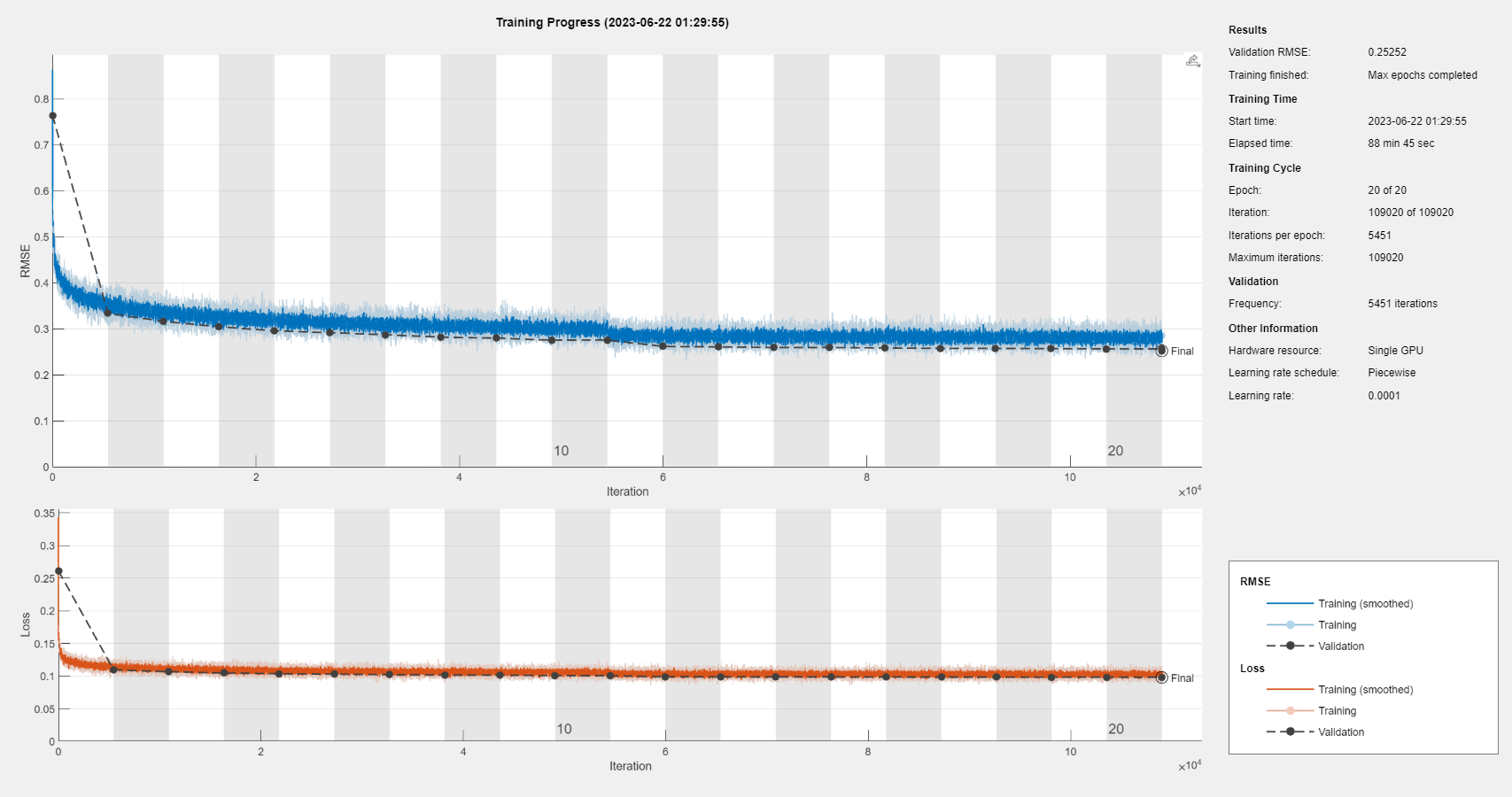
The training progress plot. Right-click for full image.

The network was trained over 20 epochs using the Adam solver. The batch size was 256. Learning rate started at 0.001 and reduced to 0.0001 after 10 epochs. L2 regularization was set to zero. Validation was done at the end of each epoch. Validation loss ended 0.0977 after 20 epochs.

The training would be several times faster if we use PyTorch/Tensorflow as the DL software, which is also more commonly used. The problem is that, unfortunately, for the next step of clustering, currently there’s no Python package that supports high dimensional (3D and above) self-organizing maps. For the sake of integrity, the project uses Matlab (R2020b or above will work) from start to end.

NN parameters

In this part I will discuss the parameters that are interpretable.

Custom activation layer

As discussed in Sec 1, this layer simulates the empirical comparison against thresholds. The training result shows most of the thresholds did not move far away from Köppen’s estimation. A notable observation is that $\sigma_{p_i}$ significantly increase with higher precipitation level $i$. This means that the network learned that overabundant precipitation rarely affect the vegetation so it deemed weaker discriminatory power on higher precipitation.

Parameter	Initial value	Learned value
$\mu_{t_1}$	-18	-16.9
$\mu_{t_2}$	0	0.6
$\mu_{t_3}$	10	10.7
$\mu_{t_4}$	22	25.3
$\sigma_t$	4	4.5
$\mu_{p_1}$	10	7.7
$\mu_{p_2}$	40	37.2
$\mu_{p_3}$	100	105.7
$\sigma_{p_1}$	10	10.0
$\sigma_{p_2}$	20	27.1
$\sigma_{p_3}$	30	59.2

fc-2 layer

This is the last layer before output that has learnable parameters. Each output neuron of this layer corresponds to a land cover type. It can be seen that predictions for deciduous needleleaf forest, closed shrubland and permanent wetland were severely suppressed by this layer. These types are relatively rare around the world. The bias parameters do not interact with the input climate data in forward propagation and thus can be seen in an average sense as indicators of impact from factors other than climate on land cover. The potential natural vegetation (Tomislav Hengl et al. 2018) may be obtained by setting these parameters to zero and then passing climate data again through the trained network, which is another topic for future exploration.

Land cover type	Cover percentage	Learned bias
evergreen needleleaf forest	2.32%	-0.19
deciduous needleleaf forest	0.32%	-1.67
evergreen broadleaf forest	6.94%	0.88
deciduous broadleaf forest	1.95%	-0.47
mixed forest	3.94%	0.27
closed shrubland	0.31%	-1.63
open shrubland	10.54%	0.31
woody savanna	8.97%	0.18
savanna	11.29%	0.15
grassland	22.38%	0.09
permanent wetland	3.87%	-1.60
cropland mosaics	8.58%	0.24
snow and ice	4.98%	-0.30
barren	13.62%	-0.28

The cover percentage in the table is based on the land cover dataset of the year 2021.

Land cover classification

The task that the neural network accomplished is to classify the climate normal data according to their underlying land cover conditions. It’s basically a multi-label classification problem. Meanwhile we hope it utilizes more information than just the label with the highest percentage (predominant land cover type), so we use the binary cross-entropy loss, expecting the NN to output the correct percentages.

In this part we reduce the problem to multi-label classification. If we see the correct label as the one with the highest percentage on the land pixel, how is the network’s performance and accuracy?

The figures are all based on the land cover dataset of the year 2021. All the maps in and after this section are of $0.5° \times 0.5°$ resolution.

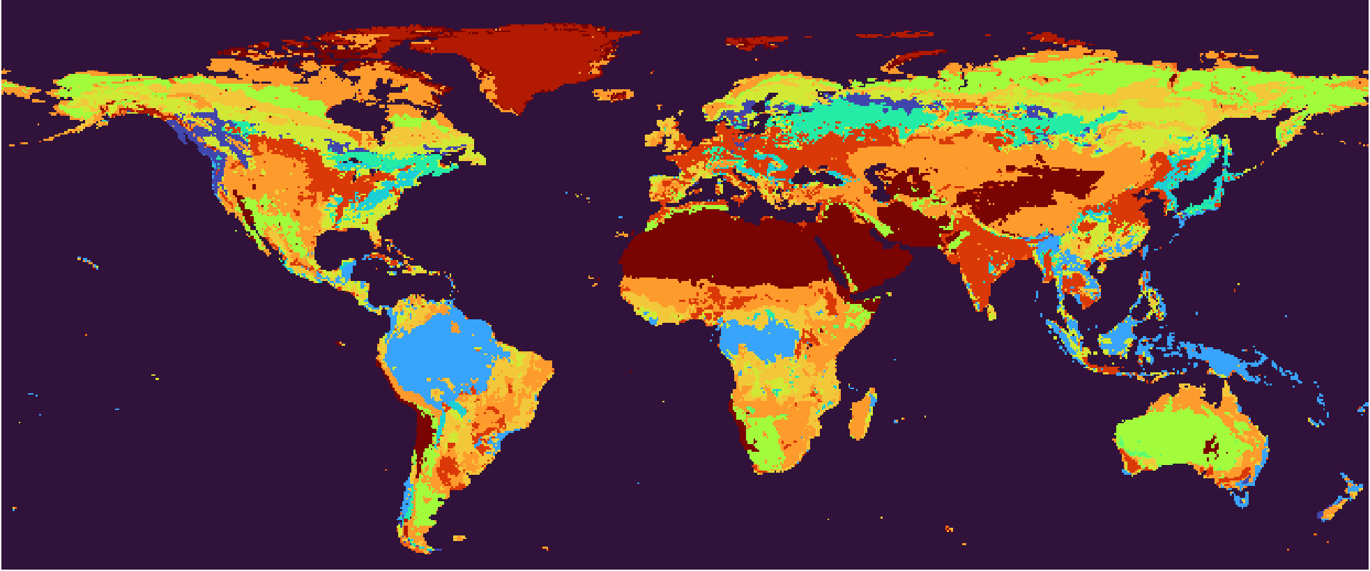Prediction target. Color each $0.5° \times 0.5°$ land pixel with its predominant land cover type, and we get the world map of land cover. Right-click for full image.

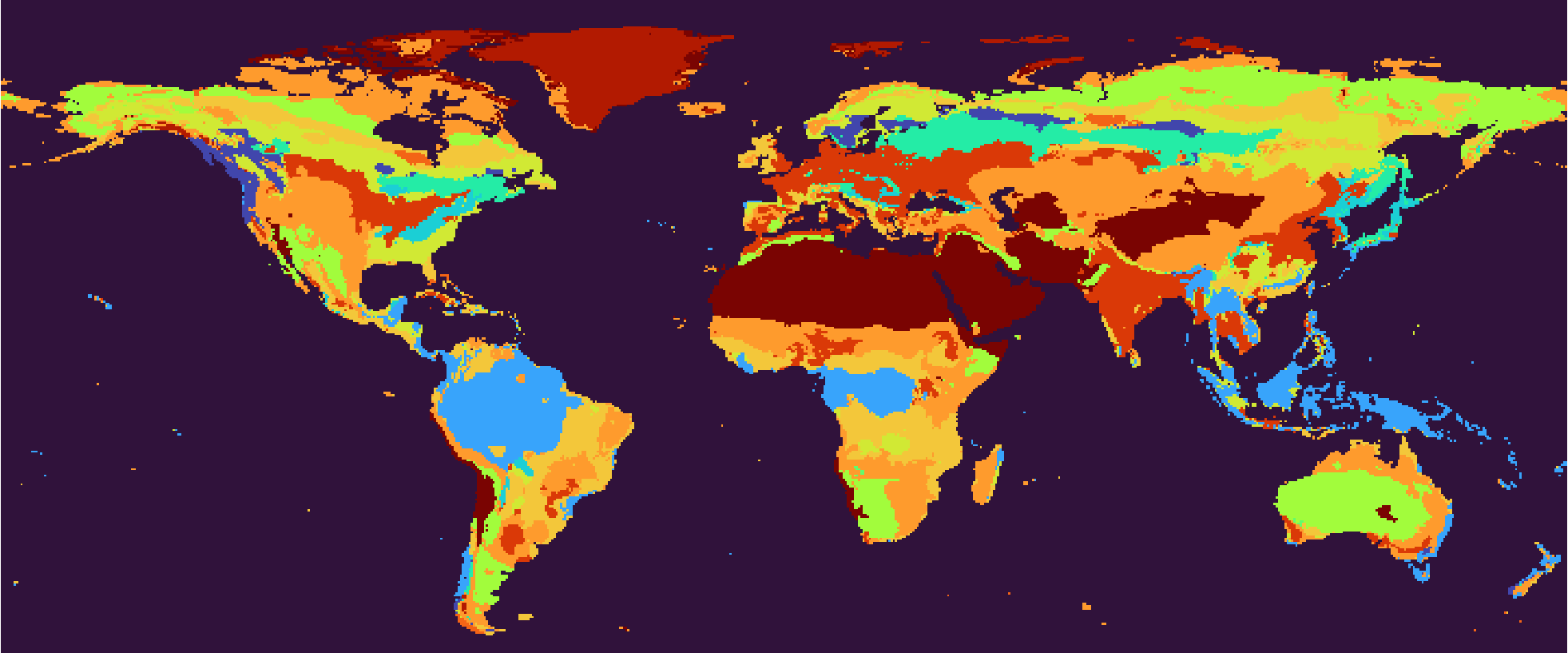Prediction output. A smoothed version of the ground truth. Right-click for full image.

Color scheme

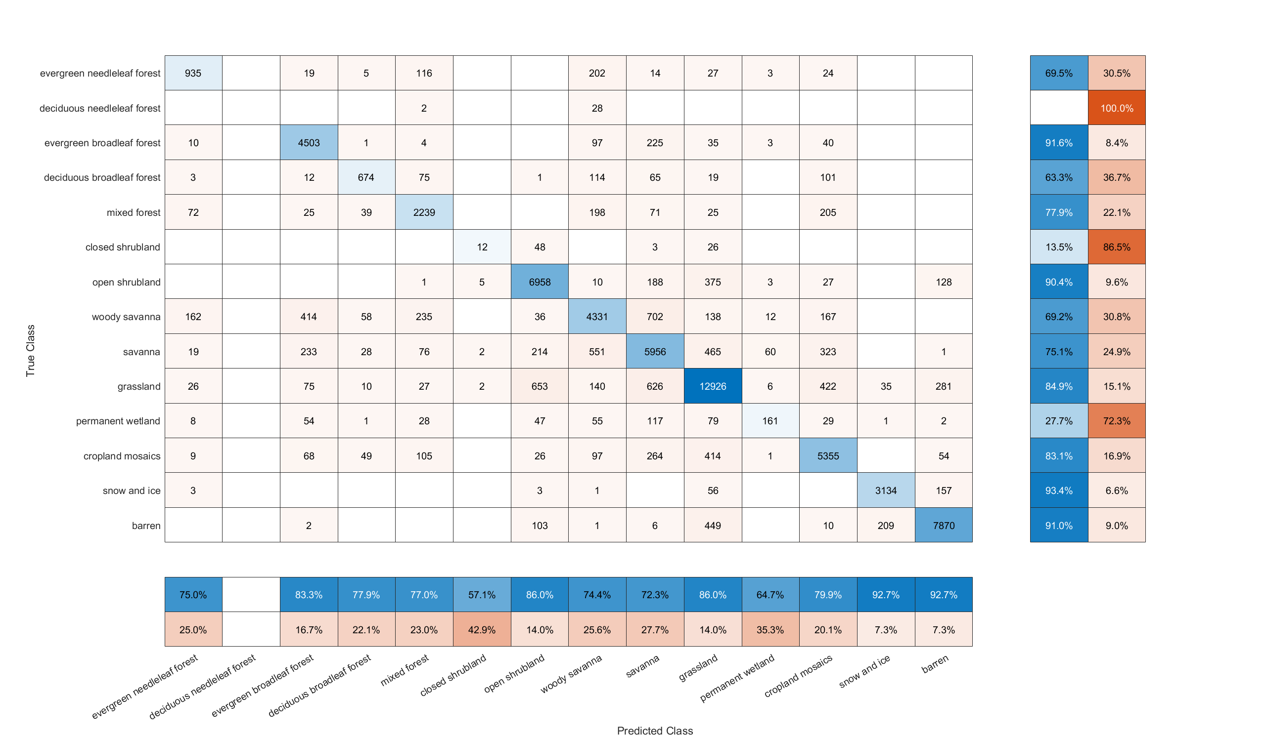Confusion chart. Right-click for full image.

From the confusion chart it can be seen that the network accurately identified land cover types such as barren and ice which are marked by pronounced climate features. Types that are underrepresented or have no clear climate features, such as closed shrubland and permanent wetland, are challenging for the network (as well as humans). The prediction achieved an overall accuracy of 82.84%. The Kappa statistic $\kappa$ is 0.8036, indicating very good agreement between real-world data and the prediction. The accuracy can be bounded by the problem’s nature: land cover is the result of multiple factors, including but not limited to climate, terrain topology and human activities. Accurate prediction of a region’s land cover merely by the local climate may imply overfitting.